
1. Introduction
1.1 What is LEGION?
LEGION is a real-time strategy game set approximately one hundred years in the future. You command large formations of autonomous electric drones across battlefields that can span up to ten kilometres on a side. There are no human soldiers on the field. Every unit, from the smallest last-mile transport drone to the massive control crawlers that anchor your logistics network, is an unmanned machine powered by battery energy.
You do not click on individual drones. You organise them into taskforces, assign those taskforces to areas of operation, and set doctrine through playbooks that govern how they behave. The drones coordinate among themselves: finding targets, allocating fire, managing their own power, and requesting resupply when they need it.
Your view of the battlefield is a tactical map in the style of a military geographic information system. Friendly units appear as NATO-standard symbology icons at their real positions. Enemy contacts appear as tracks whose detail depends on what your sensors can actually see. There is no fog of war in the conventional sense. Instead, information quality degrades naturally with distance and sensor coverage. A contact your radar lost thirty seconds ago still shows on the map, but its position estimate is bloating outward and its confidence is dropping. That distinction, between knowing where something is and knowing where it was, is central to how LEGION plays.
1.2 How LEGION Plays
LEGION has deep systems, but playing it is not complicated. At the highest level, you group units into taskforces, point those taskforces where you want them, and set doctrine that governs how they behave when they get there. The drones handle the rest: finding targets, managing power, coordinating fire, calling for resupply. A typical turn of play involves reading the map, repositioning a few taskforces, and adjusting priorities. There is no frantic clicking.
The pace is slower than most real-time strategy games. Battles unfold over minutes, not seconds. A flanking manoeuvre takes time because the units are driving across real terrain at realistic speeds. An artillery duel develops gradually as sensors refine tracks and the killweb allocates fire. You have time to think, to zoom in on a particular engagement, to check why a logistics line is stalling. The game rewards planning and positioning over reaction speed.
The depth described in this manual, the physics models, sensor equations, penetration formulas, is real, and it shapes every outcome on the battlefield. But none of it is required reading before your first game. Sensible decisions produce sensible results: put scouts in front, keep your supply lines short, do not send light drones against heavy armour. As you play more, you will naturally start noticing the patterns the simulation produces, and the deeper sections of this manual will be here when you want to understand why.
1.3 What Makes LEGION Different?
Physics, not stats
Most strategy games give units a set of authored numbers: 100 hit points, 15 damage per shot, movement speed 5. LEGION derives everything from physical first principles. A projectile penetrates armour based on its mass, velocity, material hardness, and impact angle, resolved through a real penetration model. A sensor's detection range depends on its aperture diameter, the target's cross-section, and atmospheric conditions. A unit's speed comes from its mass, motor output, and the terrain beneath it.
The practical consequence is that the game behaves the way your intuition expects. A heavier vehicle is slower but harder to push around. A bigger sensor sees further. A small drone hiding behind a hill is hard to spot not because of a "stealth" stat, but because the hill blocks line of sight and the drone has a small physical cross-section. You do not need to memorise stat tables to understand what is happening, because the simulation follows the same rules you already know from the real world.
Command, not control
You never issue orders to individual drones. You work at the taskforce level, setting objectives and doctrine. A scout taskforce told to cover an area will spread its sensor drones to maximise coverage. A combat taskforce defending a position will arrange its units to cover likely approaches and allocate fire across threats using a coordinated targeting system called a killweb.
Each taskforce's AI runs a decision cycle modelled on the OODA loop (Observe, Orient, Decide, Act), and the speed of that cycle depends on taskforce size. A four-unit recon element reacts in seconds. A forty-unit battle group takes noticeably longer to reassess and redistribute its fire. How you organise your forces matters as much as what units you build.
Logistics is the game
Every unit in LEGION runs on battery power. When a battery runs low, the unit slows down, its sensors lose range, and eventually it stops fighting. Keeping your forces supplied is not a background concern. It is a primary strategic challenge.
The logistics network is a four-tier hierarchy. Control crawlers at the back generate power and fabricate new units. Harvesters extract matter from terrain. Cargo transports shuttle charged batteries and materials forward. Last-mile drones handle the final delivery to individual units in the field. Every link in this chain can be disrupted. A flanking raid that destroys a battery crawler can stall an entire offensive without firing a single shot at a combat unit.
Deep simulation, optional inspection
Most of what happens in LEGION is invisible by default. Thousands of sensor pings, targeting calculations, power budgets, and logistics decisions execute every second beneath the map. You read the results as emergent behaviour: a formation that slows is running low on power; a track that fades has not been confirmed by sensors recently; a unit that stops advancing has taken a mobility kill.
But the simulation is not opaque. Select any unit and you can see every module's health, every sensor contact, every entry in the power budget. Select a taskforce and you can see its killweb assignments, its OODA cycle timing, and the reasoning behind its current decisions. The information is always there. It surfaces when you ask for it, not by default.
1.4 Key Concepts
These terms come up throughout the game and the rest of this manual.
| Concept | What It Means |
|---|---|
| Taskforce | A group of units operating under shared orders and doctrine. The primary unit of command. |
| Playbook | Doctrine attached to a taskforce: how aggressive it is, when it breaks contact, what it prioritises. |
| Track | A sensor contact that has been fused from multiple sources and identified to some degree of confidence. What you see on the map for enemy units. |
| Killweb | The targeting coordination system within a taskforce. Assigns weapons to targets based on range, effectiveness, and priority. |
| Module | A functional component of a unit: weapons, sensors, motors, armour plates, cargo bays, and so on. |
| Matter | The universal construction resource. Harvested from terrain or salvaged from wrecks. Used to build and repair units. |
| OODA Loop | The decision cycle of a taskforce AI: Observe, Orient, Decide, Act. Smaller taskforces cycle faster. |
1.5 How to Use This Manual
Each section covers one system and is self-contained. If you want to understand how sensors work, go to Section 5. If you want to know how to keep your forces supplied, go to Section 8. The Key Concepts table above and the table of contents at the top will help you find what you need.
Within each section, material is layered by depth:
Overview sections explain what the system does and why it matters. These are written for every player and assume no technical background.
How It Works sections go one level deeper, with concrete numbers and mechanical detail. Read these if you want to make more informed decisions about unit composition, taskforce structure, or logistics layout.
Technical Detail sections, where they appear, describe the actual simulation formulas. These are for players who want to understand exactly what the engine is computing. You will never need this information to play well, but it is there if you want it.
2. The Battlefield
2.1 The Map
LEGION presents the battlefield as a top-down military GIS display. There is no 3D rendered terrain and no fog of war. Every unit, every tracked contact, and every munition in flight exists on the same flat map surface. What varies is not whether something is visible, but how much you know about it.
Terrain elevation is shown through contour lines drawn directly on the map. Thin contour lines mark every 5 metres of elevation change; thicker index contours appear every 20 metres. Reading contours tells you where ridgelines, valleys, and slopes are before your units encounter them.
Maps are always square, ranging from 4 km to 10 km per side. A dynamic scale ruler in the corner of the display adjusts to your current zoom level so you can always judge distances at a glance.
Terrain is not just visual. It affects the simulation in two ways that directly shape your tactical options. Slope limits mobility: wheeled units cannot climb steep grades that tracked or legged units handle comfortably, and all ground units slow on inclines. Terrain also blocks line of sight. A ridge between your sensors and an enemy formation means your sensors cannot detect it, regardless of range. Positioning units on high ground gives them longer sightlines; positioning them behind a ridge hides them.
There is no satellite coverage. A cascading debris event stripped low Earth orbit clean decades before the events of LEGION, and no one has rebuilt the constellation. There is no orbital reconnaissance, no satellite relay, no GPS-precision targeting. Your entire information picture comes from sensors on your own units: cameras, radars, and the fusion systems that stitch their data together (see Section 5). If your sensors cannot see it from the ground or from low altitude, it is not on your map.
2.2 What You See on the Map

Your own units appear as NATO-style tactical icons at their actual map positions. Each icon encodes the unit's type at a glance: its frame shape indicates affiliation, interior symbols show weapon system and mission profile, a descriptor below the frame shows mobility type, and flank decorators indicate logistics roles. Section 3 covers what units are and how they work.
Enemy units are not shown directly. What you see instead are contacts and tracks produced by your sensors. A contact appears on the map only when at least one of your sensors detects the enemy unit. If no sensor can see it, it is not on your map.
When a contact first appears, it is an anonymous marker. Your sensors have detected something, but not yet gathered enough data to determine what it is. As more sensor data accumulates, the icon progressively resolves: first the contact's mobility type becomes apparent, then its weapon system and mission profile, and finally its full role classification. This progression is driven by track confidence, which Section 5 covers in depth.
Contacts that have not been updated recently by any sensor begin to desaturate, fading toward grey. This staleness indicator tells you at a glance which tracks are current and which are going stale. A fully desaturated icon means no sensor has confirmed that contact's position for several seconds. The target may have moved.
Uncertainty areas
Low-confidence contacts are surrounded by a shaded uncertainty area. This region represents where the enemy unit could actually be, given what your sensors know. A contact observed by multiple sensors from different angles has a small, tight uncertainty area. A contact seen by a single sensor, or one whose data is aging, has a larger region. The area shrinks as more sensors observe the target and grows when sensor data goes stale. High-confidence contacts (those with strong, recent sensor data) have no uncertainty area at all, indicating that your forces have a solid fix on the target.
Selecting a track highlights its uncertainty area, making it easier to assess how reliable that contact's position is. When planning engagements, the size of the uncertainty area tells you how precisely your weapons can be aimed at that target. A tight area means confident targeting. A large one means your munitions may need to search.
2.3 Taskforce Lines
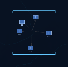
Thin lines connect each unit to its taskforce grouping, giving you a quick visual read on which units belong together. Destination lines extend from taskforces to their current movement orders, showing where each formation is headed. See Section 4 for how to organise and command taskforces.
3. Units
A unit in LEGION is an unmanned electric drone. It has a hull, a mobility system, a battery, and whatever modules you fitted to it in the unit editor. It can navigate terrain, manage its own power budget, and keep itself from crashing into obstacles. What it cannot do is decide where to look or what to shoot. Those decisions belong to the taskforce.
Think of a unit as a platform: a truck carrying sensors and guns to the right place. The sensors and guns are operated by the taskforce's coordinated systems (the sensor net, the killweb, the radar allocator), not by the unit itself. A scout drone does not choose which sector to scan. A gun platform does not pick its own target. They provide capability; the taskforce deploys it.
3.1 Anatomy of a Unit
Every unit is built from the same set of module categories, assembled from a blueprint by a fabricator.
Hull. The frame that holds everything together. Defined by width, length, and height. Hull dimensions determine the unit's physical footprint on the map, its radar cross-section (see Section 5.6), and its visual cross-section for EO detection (see Section 5.4). The hull's streamlining value affects how strongly it reflects radar energy: boxy hulls are easy to detect, faceted hulls scatter radar, smooth hulls fall between. Armour can be fitted to the hull to absorb damage.
Mobility. How the unit moves. Five types exist: wheeled, tracked, legged, fixed rotor, and tilt-axis rotor. Each has different speed, terrain access, and energy characteristics. See Section 3.2.
Sensors. EO cameras and radar arrays mounted on the hull. The unit carries them; the taskforce operates them. A unit might carry one EO sensor and one radar, or three radars and no EO, or any other combination. The taskforce's sensor allocation and radar mode assignment decide how each sensor is used at any given moment.
Turrets. Weapon mounts: guns, missile launchers, lasers, CIWS. A turret belongs to the unit physically (it rotates on the hull, draws power from the battery, takes damage when hit) but is aimed and fired by the taskforce's killweb. The unit has no say in target selection.
Battery bay. Energy storage. A single pool powers everything: movement, sensors, radar, weapons. When the battery runs low, performance degrades across the board. See Section 3.3.
Support modules. Supply bays for carrying spare batteries and materials, docking bays for hosting smaller drones, external cargo racks. These enable logistics roles (see Section 8).
3.2 Mobility
Wheeled. Fast on flat terrain and roads. Poor slope tolerance; steep hills force long detours. Light and cheap to build. Best for flat operating areas where speed matters more than terrain access.
Tracked. Moderate speed with good slope tolerance. Heavier and more expensive than wheeled, but climbs grades that wheels cannot. The default choice for combat units that need to go most places.
Legged. Slow, but excellent slope tolerance. Legged units traverse terrain that stops everything else: steep ridges, rocky escarpments, broken ground. Expensive and power-hungry. Worth it when the terrain demands it or when you need a position only legs can reach.
Fixed rotor. Ignores terrain entirely. Flies in three dimensions, limited by power consumption. Hovering costs energy even when stationary. Higher altitude extends sensor range but makes the unit more visible to enemy EO (see Section 5.4). Fast and agile but drains batteries quickly.
Tilt-axis rotor. Hybrid: takes off and lands vertically like a rotorcraft, then transitions to forward flight for efficient cruising. More complex and heavier than a fixed rotor, but substantially more energy-efficient at speed.
Speed is not an authored number. It emerges from the unit's motor power, mass, drag, and terrain. A heavier unit with the same motor is slower. A unit climbing a slope is slower than one on flat ground. You control the inputs (motor size, hull weight, mobility type) and the physics produces the speed.
3.3 The Energy Budget
Every unit has a single battery pool. Movement, sensors, radar, and weapons all draw from the same energy reserve. There is no separate fuel tank or ammunition supply; it is all electricity.
Movement is typically the largest draw. Faster movement costs more power. Rotorcraft burn energy to maintain altitude even when hovering in place. Climbing a slope costs more than crossing flat ground. Legged units are particularly power-hungry due to the mechanical complexity of their gait.
Radar is the second largest draw for units that carry it. Point Defence mode costs twice the baseline power. Surveillance is moderate. Track mode is efficient, drawing only half the baseline. Choosing how many radars to field in a taskforce is partly an energy budget decision.
Weapons draw from the same pool. Lasers are the most energy-intensive: sustained beam fire drains the battery fast. Kinetic weapons (guns, railguns) draw less per shot. Missiles draw only at launch.
When the battery runs low, everything degrades. Speed drops. Sensor range shortens. Eventually the unit stops moving and fighting. A unit with a dead battery is a stationary, defenceless target. Resupply comes from the logistics network: transport drones deliver charged battery cells to units in the field (see Section 8).
The all-electric design is not a stylistic choice. Batteries charged from a fusion reactor deliver roughly three times more useful work per joule of reactor energy than synthesising fuel and burning it. The efficiency gap is set by thermodynamic law, not engineering limitations, so no amount of future technology closes it. Combustion still appears in expendable applications (missile propellant, short-burn boost phases) where the energy cost is small and one-time. Sustained propulsion is electric because the alternative is wasteful to the point of being operationally indefensible.
This is why all aircraft in LEGION are electric rotorcraft (tiltrotors, ducted-fan VTOL platforms) rather than jet-powered fixed-wing aircraft. Jet engines need fuel, and printing fuel on the battlefield costs three times more reactor energy than charging batteries for the same flight time.
Why not jet fuel?
The matter printers that fabricate units can synthesise hydrocarbon fuel. The technology exists. It is not used for sustained propulsion because the thermodynamics make it ruinously wasteful.
Energy reaches a unit through one of two pathways. The electric pathway runs from the control crawler's fusion reactor through a charging station into battery cells, then from battery to motor. Each step is highly efficient: power distribution (~95%), charging (~97%), discharge and power electronics (~94%), motor (~96%). The total chain delivers roughly 84% of the reactor's input energy as mechanical work at the wheels or rotors.
The fuel pathway adds two punishing steps. First, the matter printer must synthesise hydrocarbon fuel from raw feedstock. This is an inherently lossy process: constructing chemical bonds costs energy that cannot be recovered, side reactions waste more, and purification costs more still. Even an advanced 2100-era printer achieves roughly 65% efficiency from electrical input to chemical energy stored in the fuel. Second, the fuel must be burned in a heat engine, and every heat engine is capped by the Carnot limit: no matter how good the turbine, roughly half the fuel's energy is rejected as waste heat. A realistic advanced turbine converts about 49% of fuel energy to shaft power.
Multiply through the fuel chain (95% distribution, 65% synthesis, 49% combustion, 95% mechanical) and roughly 29% of the reactor energy reaches the point of use. Compare that to 84% for the electric chain. For the same four-hour rotorcraft patrol, the fuel pathway consumes nearly three times more reactor energy, and the surplus is dumped as waste heat at the printer and the engine exhaust.
Neither the synthesis floor nor the Carnot ceiling can be engineered away. They are consequences of thermodynamic law. The electric pathway avoids both: it never synthesises fuel (no synthesis losses) and never burns it (no Carnot limit). In a setting where reactor output is the binding logistical constraint, spending three joules to do one joule of work is a luxury no commander can afford.
3.4 Fabrication
Units are built by control crawlers from raw matter and energy. You design a blueprint in the unit editor, queue it for production, and the fabricator assembles it. Building requires matter (harvested from terrain) and energy (drawn from the same power grid that runs everything else).
Bigger, heavier units cost more matter and take longer to build. A small scout drone is cheap and fast. A large combat platform with thick armour and multiple turrets is expensive and slow to produce. A fabricator running at full capacity competes with radar, sensors, and weapons for energy, so building new units during a fight has a real cost beyond just the matter.
Losses matter because replacement takes time. A unit destroyed in the field is not just a piece removed from the board; it is minutes of fabrication time that cannot be recovered. Preserving your units through good positioning, timely resupply, and avoiding unnecessary engagements is often more valuable than building replacements.
3.5 Unit Classification
Every unit in LEGION receives a classification label when it is assembled. This label is not hand-assigned; it is derived from the unit's actual physical properties. A tracked chassis with a high-penetration gun and thick armour is classified as a Tank. Swap the gun for a sensor array and the label changes to Scout. The classification reflects what the unit is, computed from what it has.
You can see a unit's classification in the unit editor and in the details panel during play. The label is your at-a-glance summary: it tells you the unit's primary role and any notable secondary strengths without requiring you to inspect every module individually.
The Capability Vector
Behind the label is a capability vector: eight scores, each measuring a different aspect of what the unit can do.
| Dimension | What It Measures |
|---|---|
| Firepower (Direct) | Sustained damage output from guns, railguns, and other direct-fire weapons. Measured in HP per second. |
| Firepower (Indirect) | Sustained damage output from guided missiles and other indirect-fire weapons. Measured in HP per second. |
| Anti-Air | Effectiveness against aerial targets, accounting for turret elevation, traverse speed, and engagement range. Also covers close-in point defence against missiles. |
| Survivability | Total hit points from armour plates and internal structure. |
| Speed | Top speed on flat terrain, in metres per second. |
| Recon | Sensor coverage, weighted by range. Radar sensors contribute more than optical sensors of equal range. |
| Logistics | Cargo and transport capacity: supply bay cells, docking bay volume, external cargo payload, and matter tank capacity. |
| Stealth | How hard the unit is to detect, combining low radar cross-section with a small visual profile. Ranges from 0 (conspicuous) to 1 (nearly invisible). |
Every value is derived from the unit's modules at assembly time. Fitting a larger motor raises speed. Adding armour raises survivability but may lower speed (more mass, same motor). Mounting a radar dish raises recon but lowers stealth (larger cross-section). The capability vector makes these tradeoffs visible.
Capability Glyphs
The capability vector is displayed as a capability glyph wherever unit details appear: the unit editor, the selection details panel, and taskforce composition views. Each wedge represents one CV dimension. The size of the wedge shows the unit's strength in that dimension relative to its other scores, so you can read a unit's role at a glance from the shape of the glyph.
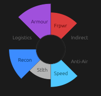
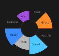
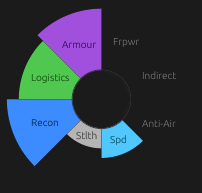
A tank's glyph is heavy on the Armour and Firepower wedges. A scout's glyph is dominated by Recon. A logistics crawler's glyph peaks on Logistics and Speed. Two units with similar labels but different glyph shapes have meaningfully different capability profiles, and the glyph makes that difference visible without reading numbers.
How Labels Are Built
A classification label has two parts: a noun and up to two adjectives.
The noun comes from the unit's strongest capability dimension crossed with its mobility type. A tracked unit whose dominant dimension is direct firepower is a Tank. A wheeled unit dominated by recon is a Scout Car. A legged unit with high logistics capacity and docking bays is a Carrier.
Some nouns require multiple dimensions to be strong simultaneously. A unit only earns the Tank label if it has both high direct firepower and high survivability, with a weapon heavy enough to qualify as a tank gun rather than an autocannon. A unit classified as a CIWS Vehicle has a turret physically suited to intercepting incoming missiles: fast traverse, high fire rate, and accurate projectiles.
Adjectives layer on secondary strengths. A tank with unusually high speed becomes a Fast Tank. A scout with significant armour becomes a Heavy Scout Car. The possible adjectives are Heavy (high survivability), Fast (high speed), Armed (significant firepower), AA (anti-air capability), Recon (good sensors), and Stealth (low signature). A unit gets at most two; they are ranked by strength and only the top two appear.
Classification Examples
| Mobility | Dominant Strengths | Classification |
|---|---|---|
| Tracked | High direct firepower, thick armour, heavy gun | Tank |
| Tracked | High direct firepower, thick armour, heavy gun, fast | Fast Tank |
| Wheeled | Strong sensors, light armour | Scout Car |
| Wheeled | Strong sensors, decent stealth | Stealth Scout Car |
| Legged | High indirect firepower | Artillery Mech |
| Legged | High indirect firepower, thick armour | Assault Mech |
| Tracked | Fast-tracking turret, high fire rate, anti-air DPS | CIWS Vehicle |
| Wheeled | Direct firepower, light armour | Gun Truck |
| Fixed Rotor | High direct firepower | Gunship |
| Fixed Rotor | High indirect firepower | Bomber |
| Fixed Rotor | Strong sensors | Scout |
| Tracked | Supply bays, matter tank | Cargo Crawler |
| Legged | Docking bays | Carrier |
| Wheeled | Large external cargo racks | Transport |
| Tracked | Heavy armour, minimal weapons | Fortress |
Because classification is derived from physics, changing a single module can shift a unit's label. Replacing a tank's main gun with a missile launcher turns it from a Tank into Artillery. Stripping armour off a Fortress until its sensor score dominates reclassifies it as a Scout. The label always reflects the unit you actually built, not the one you intended.
3.6 Damage and Degradation
Damage in LEGION does not flip a switch from "working" to "destroyed." It degrades capability. A turret with a damaged drive mechanism still traverses, just slower. A sensor with cracked optics still detects, just at shorter range. An engine losing power output makes the unit sluggish, not immobile. Destruction is the end state, but between full health and destruction there is a wide range of partial capability where a damaged unit is still useful, just less so.
Every module on a unit has an effectiveness value between 0 and 1. A healthy module sits at 1.0. As it takes damage, effectiveness drops along a curve that is forgiving at first: a module at 50% hit points still operates at roughly 70% effectiveness. The degradation accelerates as damage accumulates. A module at 25% HP is down to 50% effectiveness, and below that it falls off sharply.
How Modules Degrade
| Module | Effect of Reduced Effectiveness |
|---|---|
| Engine | Peak torque and max RPM scale directly. A damaged engine means lower top speed and weaker hill climbing. |
| Turret | Horizontal and vertical traverse rates scale with effectiveness. A badly damaged turret tracks targets slowly. Below 10% effectiveness, the turret locks in place; it can still fire at whatever it happens to be pointing at, but it cannot track. |
| Sensor (Radar) | Detection range scales with the square root of effectiveness. A radar at 50% effectiveness retains roughly 70% of its rated range. |
| Sensor (Optical) | Detection range scales with the square root of effectiveness, same as radar. |
| Battery Bay | Discharge rate scales directly. A damaged battery bay delivers power more slowly, starving energy-hungry modules. |
| Capacitor | Both charge and discharge rates scale directly. A damaged capacitor charges and delivers energy more slowly. |
| Printer | Print rate scales directly. Below 5% effectiveness, printing stalls entirely. In-progress jobs pause but do not fail; they resume if the printer recovers. |
| Weapon | Fire rate scales directly. Below 10% effectiveness, the weapon is disabled entirely and will not fire. |
| Docking Bay | Binary. Below 10% effectiveness, the bay is disabled: it cannot accept or release docked units. Units already docked are unaffected. |
Energy starvation compounds the problem. If the battery bay is damaged and cannot deliver enough power, modules that demand energy operate at reduced effectiveness even if they are physically undamaged. A unit with a crippled battery bay degrades across the board.
Mobility Damage
Mobility substructures (tracks, wheels, legs, rotors) feed their average effectiveness into an overall traction or thrust capacity. Damaged substructures contribute less; destroyed ones contribute nothing. A four-legged walker with one leg at half effectiveness and three healthy ones still has roughly 88% traction.
Tracked vehicles face catastrophic failure. When a track's HP drops below 50%, there is a growing chance per second that the track link fails entirely. The probability ramps from rare to near-certain as HP approaches 25%. A single thrown track drops the vehicle's traction to 10% of normal, regardless of the state of other tracks. The vehicle can still crawl, but it is effectively immobilized for tactical purposes.
Legged units have a different failure mode. Legs risk structural breakage below 30% HP, with probability ramping up toward 20% HP. A broken leg contributes nothing to traction. If half or more of a unit's legs are broken, traction drops to zero: the unit is fully immobilized. A six-legged walker can lose two legs and keep moving (at reduced speed); losing a third stops it entirely.
4. Taskforces
A taskforce is the fundamental unit of agency in LEGION. It is the only thing you command. You do not give orders to individual units; you give orders to taskforces, and the taskforce coordinates its units to carry them out.
A taskforce is not a selection group. It is a distributed organism. The units are its body: they carry the sensors, weapons, and logistics capacity to the right positions. The taskforce's coordinated systems are its brain: the sensor net fuses every camera and radar across every unit into a single intelligence picture; the killweb assigns every turret across every unit to targets from that picture; the radar allocator distributes scan modes across every radar in the formation. A turret on one unit might be shooting at a target that a sensor on a different unit detected. The units do not know or care. They provide the hardware; the taskforce provides the coordination.
How you divide your forces into taskforces is one of the most consequential decisions in the game.
4.1 Movement and Pacing
When you order a taskforce to move, it advances toward the destination at roughly half the maximum speed of its slowest unit. The formation holds together automatically: units spread out within the group and keep pace with each other.
If too many units fall behind, the taskforce slows down and waits for stragglers to catch up before resuming its advance. You do not need to babysit spacing; the taskforce manages its own cohesion.
Ground taskforces follow terrain-aware paths that respect slope limits. The slope limit is set by the unit in the roster with the worst climbing ability. A taskforce containing both wheeled vehicles (poor slope tolerance) and legged walkers (excellent slope tolerance) will route around hills that the walkers could climb alone. If you need units to take different routes, split them into separate taskforces.
Air-only taskforces (containing only rotorcraft or tilt-rotors, no ground vehicles) ignore terrain entirely. They advance in a straight line toward the destination at the speed of their slowest member.
4.2 Sensors and the Track List
Every sensor on every unit in the taskforce feeds into a shared sensor net. A scout drone's radar and a tank's EO camera contribute to the same intelligence picture. The taskforce fuses all contacts into a single track list: a filtered subset of the side-wide sensor picture containing only the tracks spatially relevant to the formation.
The track list is refreshed on an OODA tick, a periodic decision cycle whose speed depends on the taskforce's size. A small taskforce of five units refreshes its tracks roughly every 1.5 seconds. A large taskforce of thirty units takes about 4 seconds between refreshes. Smaller taskforces detect changes faster and can reassign weapons sooner. Larger taskforces bring more sensors and more firepower, but their collective decision-making is slower.
4.3 Fire Control: The Kill Web
The kill web is the taskforce's automated fire coordinator. It surveys every turret across all units in the taskforce and assigns each one a target from the track list. A turret on unit A might be assigned a target that unit B's sensor detected halfway across the formation. The units are interchangeable weapon platforms; the killweb treats the entire taskforce as a single distributed weapons system.
Standard turrets (guns, missiles, lasers) are assigned through a priority system that considers penetration capability against the target's armour, range, and how many other turrets are already engaging that target. The kill web prefers to match weapons to targets they can actually hurt: a light autocannon will not be wasted on a heavily armoured tank if softer targets are available, and a heavy railgun will not be pointed at a drone when there is armour to crack.
Close-in weapon systems (CIWS) use a different algorithm tuned for missile defence. Incoming missiles are grouped into clusters based on their direction and proximity, and CIWS turrets are assigned to clusters rather than individual missiles. This ensures point defence covers threat axes evenly rather than chasing individual projectiles.
4.4 Radar Allocation
Taskforces with radar-equipped units automatically distribute radar modes across their sensors each OODA tick. The allocation treats every radar in the formation as part of a single coordinated array. Three modes are assigned in priority order. Track maintenance comes first: radars are aimed at existing tracks to keep their position estimates accurate, prioritising the lowest-confidence tracks. Surveillance comes second: at least one radar is kept in a 360-degree sweep (the one with the best base range is chosen). Search fills the remainder: unassigned radars are oriented toward the bearing sectors that have gone longest without a scan.
You do not control radar modes directly. The allocation is automatic and responds to the tactical situation. A taskforce with many tracked contacts will devote more radars to track maintenance. One with few contacts will spread radars across search sectors to build situational awareness.
4.5 Composition and Tradeoffs
Because movement speed, slope routing, OODA cadence, fire control, and radar allocation all operate at the taskforce level, the mix of units you put in a taskforce shapes its behaviour in ways that are not always obvious.
Speed is limited by the slowest member. Adding a single logistics crawler to a taskforce of fast scout drones means the entire group moves at crawler speed. Slope tolerance is limited by the worst climber. Reaction time grows with roster size. Fire control works best when there are enough weapons to spread across available targets, but diminishing returns set in as the kill web has more turrets than it has worthwhile targets for.
When you design a taskforce composition, you are assembling a distributed system. The sensors, weapons, and logistics capacity of individual units combine at the taskforce level into something greater than the sum of its parts. A formation with overlapping sensor coverage, diverse weapon types, and enough logistics to sustain itself is resilient. One that depends on a single sensor unit or a single weapon platform has a single point of failure.
5. Sensors and Detection
Without sensors, the battlefield is dark. You cannot target what you cannot see, and your taskforce AI cannot react to threats it does not know about. Sensors are how your force turns the unknown into actionable intelligence.
5.1 Sensor Overview
Every unit in LEGION carries one or more sensors. A unit can mount several sensors of different types, and each operates independently with its own scan rate, range, and detection characteristics.
There are two sensor modalities. Electro-optical (EO) sensors are passive cameras that detect targets by their visual signature. Radar sensors are active emitters that bounce radio waves off targets and listen for the return. A unit might carry both: an EO sensor for passive awareness and a radar for long-range active detection. Each type has different strengths, different blind spots, and different ways of computing how well it can see a target.
Detection is not binary. Each sensor contact has a quality score between 0 and 1. A faint contact at long range in haze might register at 0.05, too low to act on. A large target at close range on a clear day might register at 0.9, enough to identify the target's weapon system. Contacts below a sensor's detection threshold are discarded. Everything above it contributes to your force's shared intelligence picture.
5.2 How Detection Works
Each sensor determines what it can see based on range, line of sight, and its own arc of coverage. A target behind a hill is invisible regardless of range. For each target a sensor can see, it computes a quality score that reflects how clearly it can resolve that target. The quality model is different for each sensor type: EO quality depends on the target's visual cross-section, distance, atmospheric conditions, speed, and altitude; radar quality depends on the target's radar cross-section, Doppler shift, and the inverse fourth power of range. The details of each model are covered in the sensor-specific sections below.
Sensors with higher scan rates update more often. With many units on the field, individual sensors may occasionally skip a cycle, but higher-priority sensors are serviced first.
5.3 From Contacts to Tracks
Individual sensor contacts are short-lived. The fusion system aggregates them into tracks: persistent records of an enemy's estimated position, velocity, and identity. Each contact contributes a position estimate with an uncertainty region. Range is harder to judge than bearing, so the uncertainty is elongated along the line of sight. A high-quality contact produces a small, tight region; a low-quality one produces a large, vague area.
When multiple sensors observe the same target, their uncertainty regions overlap and the track's position estimate tightens. The estimated position is a quality-weighted average of all contributing observations. The track's confidence score reflects how tightly constrained the position is. The fusion system also estimates target velocity from successive observations.
Position uncertainty grows over time at a rate proportional to the target's estimated speed. If no sensor refreshes a track, the uncertainty eventually exceeds 500 metres and the track is dropped. Tracks older than 30 seconds fade: their confidence decays linearly to zero. The killweb and taskforce AI both use confidence to filter which targets are worth engaging.
Classification
When a sensor first detects a target, the contact is classified as Unknown. As the contact quality improves, the classification progresses through three stages.
Partial identification occurs at a quality of 0.2. You learn the target's mobility type: wheeled, tracked, legged, or rotorcraft. Enough to distinguish a tank from a helicopter, not enough to know what weapons it carries.
Full identification occurs at a quality of 0.5. The target's weapon system and mission profile become visible. You can now tell the difference between a missile truck and a supply crawler.
Detailed identification occurs at a quality of 0.7. The target's logistics role is revealed, completing the picture.
Classification is permanent: once a target has been identified, its identity does not degrade even if the sensor loses contact. Only the track's position confidence degrades over time.
Track distribution
Tracks are distributed to taskforces based on spatial relevance. Each taskforce sees tracks within its weapon range plus a margin, drawn from the side-wide track table. A taskforce does not need its own sensors to act on a track, but tracks from other taskforces' sensors carry less local certainty.
5.4 Electro-Optical Sensors
EO sensors are passive cameras. They emit nothing and cannot be detected by the enemy. Every standard unit carries at least one. Their maximum range is limited by the horizon: a ground vehicle sees to about 5,000 metres, while a rotorcraft at altitude can see much further.
EO detection depends on conditions. A stationary target can be invisible at ranges where a moving one is obvious. Haze degrades range. A narrow silhouette (head-on or tail-on) is harder to resolve than a broadside profile. Targets silhouetted above the horizon (rotorcraft, hilltop positions) are easier to spot.
Speed has a surprising effect. A target that stops moving can vanish from EO entirely. A target moving at typical combat speeds is easy to see. A very fast target (above 50 m/s) actually becomes harder to resolve, and by 100 m/s the speed bonus drops to zero. A fast rotorcraft dash can reduce your EO signature, though radar will still see you.
5.5 EO Detection Model
This section provides tools and formulas for understanding EO detection in depth. The explorer lets you experiment with scenarios interactively, the technical detail documents the exact formulas, and the worked example walks through a concrete calculation step by step.
5.5.1 EO Detection Explorer
Understanding EO Sensors In Depth
The four factors
Four factors combine to determine EO detection quality:
Apparent size. The target is modelled as a 3D box. The visible cross-section depends on which faces the observer can see. Head-on viewing shows the narrow front face (width times height). Broadside shows the full side (length times height). This cross-section is compared to the sensor's reference area (14 m^2 by default). A target with a larger cross-section is easier to detect.
Distance. The apparent size of a target falls as the inverse square of distance. At the reference range of 1,500 metres, a reference-sized target has a size factor of 1.0. At 3,000 metres it drops to 0.25. At 6,000 metres, 0.0625.
Speed and altitude bonuses. Moving targets are easier to spot. Below 2 m/s the target is treated as stationary (no bonus). The bonus ramps smoothly to full strength at 6 m/s and holds through typical combat speeds up to 50 m/s. Above 50 m/s it drops back toward zero, reaching zero at 100 m/s. Targets above 10 metres altitude gain an additional bonus (up to 0.5) because they are silhouetted against the sky rather than blending with terrain.
Atmospheric haze. Haze attenuates the signal exponentially with distance. At the default visibility of 15,000 metres, transmittance drops to about 2% at that distance. Closer targets lose much less signal. At 4,000 metres, roughly 35% of the signal survives.
Scan rate and horizon
EO sensors scan at 10 Hz. Their maximum range is the geometric horizon, which depends on observer altitude: roughly 5,000 metres at ground level, extending to about 35,700 metres at 100 metres altitude. Beyond the horizon, detection quality is zero regardless of target size or speed.
5.5.2 Technical Detail: Formulas
Visible cross-section
The target is modelled as an axis-aligned box with dimensions width (W), length (L), and height (H), taken from the visual envelope if turrets or legs extend beyond the hull, or from the hull shape otherwise. The view direction V is the unit vector from observer to target. The visible cross-section is the sum of three face-pair projections:
cross_section = W * H * |V . forward| + L * H * |V . right| + W * L * |V . up|
where forward, right, and up are the target's local axis unit vectors. Head-on viewing maximises the front-back term (W * H) while minimising the side term. Broadside maximises L * H. Viewing from above maximises W * L.
Size factor and perspective
The size factor normalises the cross-section against the sensor's reference area (14 m^2 by default) and applies perspective falloff:
size_factor = (cross_section / reference_area) * min(1, (ref_range / distance)^2)
The reference range is 1,500 metres. At distances shorter than the reference range the perspective term is capped at 1.0 (the target cannot appear larger than its actual cross-section). Beyond 1,500 metres, the signal falls as the inverse square of distance.
Observability bonuses
Speed and altitude bonuses are added to the size factor before atmospheric attenuation.
The speed bonus follows a band-shaped curve. Below 2 m/s the bonus is zero. It ramps up via a smooth curve to 1.0 at 6 m/s, holds at 1.0 through typical combat speeds up to 50 m/s, then ramps back down to zero at 100 m/s. The ramps use a smooth ease-in-out (cubic smoothstep) rather than a hard linear transition. Expressed as a piecewise function:
speed_bonus(v) =
  0                                       if v <= 2
  smoothstep((v - 2) / 4)                 if 2 < v < 6
  1                                       if 6 <= v <= 50
  smoothstep((100 - v) / 50)              if 50 < v < 100
  0                                       if v >= 100
where smoothstep(t) = t^2 * (3 - 2t) and v = |speed| in m/s.
Altitude bonus activates above 10 metres AGL and ramps linearly to a maximum of 0.5 over a 50-metre range (reaching maximum at 60 metres AGL).
Atmospheric transmittance
Atmospheric extinction follows Beer-Lambert: transmittance = exp(-sigma * distance), where sigma = 3.912 / meteorological_visibility. At the visibility distance, transmittance drops to exp(-3.912), approximately 0.02 (the standard 2% threshold that defines meteorological visibility). The default visibility is 15,000 metres.
Final quality
quality = clamp(0, 1, (size_factor + speed_bonus + altitude_bonus) * transmittance)
A contact with quality below the detection threshold (0.1) is discarded. Contacts above the threshold are passed to the fusion system.
Horizon distance
The maximum detection range for an EO sensor is the geometric horizon:
horizon = sqrt(2 * R_earth * observer_AGL)
where R_earth = 6,371,000 metres. Observer AGL is the sensor's height above the terrain surface: the unit's Z position (or the terrain height, whichever is greater) plus the shape offset Z plus the shape height. For a ground unit with a sensor at 2 metres AGL, the horizon is about 5,048 metres. For a rotorcraft at 100 metres AGL, approximately 35,700 metres.
5.5.3 Worked example: scout rotorcraft detecting a medium tank
A scout rotorcraft at 80 metres AGL observes a medium tank (width 3.5m, length 7.0m, height 2.5m) at 4,000 metres, broadside-on, in clear weather (visibility 15,000m). The tank is moving at 12 m/s.
Visible cross-section. Broadside viewing means the view direction is roughly perpendicular to the tank's forward axis. The dominant face is the side: L * H = 7.0 * 2.5 = 17.5 m^2. The front/back and top contributions are near zero at this angle. Cross-section is approximately 17.5 m^2.
Size factor. The sensor's reference area is 14 m^2. The reference range is 1,500m. At 4,000m the perspective term is (1500 / 4000)^2 = 0.141. Size factor = (17.5 / 14) * 0.141 = 0.176.
Speed bonus. The tank moves at 12 m/s, well within the full-bonus band (6 to 50 m/s). Speed bonus = 1.0.
Altitude bonus. The tank is on the ground (0m AGL), below the 10m threshold. Altitude bonus = 0.
Atmospheric transmittance. Sigma = 3.912 / 15000 = 0.000261. Transmittance = exp(-0.000261 * 4000) = exp(-1.044) = 0.352.
Final quality. (0.176 + 1.0 + 0) * 0.352 = 0.414. Above the detection threshold of 0.1. At this quality, the tank is partially identified (mobility type visible at 0.2), but not yet fully identified (requires 0.5).
What if the tank were head-on? The dominant face becomes W * H = 3.5 * 2.5 = 8.75 m^2. Size factor drops to (8.75 / 14) * 0.141 = 0.088. Final quality = (0.088 + 1.0) * 0.352 = 0.383. Still detected at 4,000 metres. Both orientations drop below detection at roughly 8,900 metres; at full speed bonus the cross-section difference barely matters because the bonus dominates the signal. The concealment advantage of a narrow profile only shows at long range where the size factor is the deciding term.
What if the tank were stationary? Any speed below 2 m/s produces zero speed bonus. Quality = 0.176 * 0.352 = 0.062. Below the 0.1 threshold. A stationary tank at 4,000 metres broadside-on is invisible to this sensor. Solving for the detection boundary: a stationary broadside tank becomes detectable at roughly 3,400 metres. Head-on and stationary, that drops to about 2,650 metres.
What about extreme speed? A rotorcraft crossing the field at 80 m/s (288 km/h) has a reduced speed bonus of 0.35. At 4,000 metres broadside, quality drops to (0.176 + 0.35) * 0.352 = 0.186. Still detected, but substantially harder to resolve than the same target at 30 m/s. At 100 m/s the speed bonus is zero and the rotorcraft relies entirely on its cross-section, just like a stationary target.
Why this matters to you: a unit that stops moving is not just harder to detect, it can be genuinely invisible at ranges where the same unit in motion would be an easy contact. Holding position in cover is not a marginal advantage; it is the difference between being seen and not being seen. At the other extreme, a fast rotorcraft or missile that crosses the field above 50 m/s starts to become optically harder to resolve, and above 100 m/s it vanishes from EO entirely (radar is another matter). A stationary force behind a ridge can let an enemy taskforce pass within 3 kilometres without appearing on their EO picture, then engage from a range the enemy never expected.
5.6 Radar Sensors
Radar is active: it transmits energy and listens for the return. It sees further than EO and works through haze, but it has a critical blind spot: it cannot detect stationary targets. If a target is not moving toward or away from the radar, it is invisible. A target crossing perpendicular to the radar beam is equally invisible, regardless of speed.
EO and radar are complementary. EO sees stationary ambushes that radar misses. Radar sees fast movers at long range that EO cannot resolve through haze. A taskforce with both sensor types covers both blind spots. A taskforce with only one will be surprised by the threats the other would have caught.
Radar range drops steeply with distance. A target at twice the range returns one sixteenth the signal. Bigger antennas and more power extend range, but at a cost: radar drains battery energy while active. The taskforce automatically assigns each radar to a mode (see Section 4.4) that balances coverage, range, and power draw.
How visible a target is to radar depends on its size, hull shape, and the angle it presents. Boxy hulls reflect strongly. Faceted hulls with angled surfaces scatter radar energy away. A target seen broadside returns more signal than one seen head-on.
5.7 Radar Detection Model
This section provides tools and formulas for understanding radar detection in depth. The explorer lets you experiment with detection scenarios, the technical detail documents the formulas, and the worked example walks through a calculation.
5.7.1 Radar Detection Explorer
Understanding Radar In Depth
Radar cross-section
A target's radar visibility depends on its radar cross-section (RCS): how strongly it reflects radar energy back toward the emitter. RCS is driven by two factors. Physical size sets the baseline: a larger hull presents more surface area to reflect from. Hull shape modifies the baseline: a boxy hull with flat panels and sharp corners acts as a collection of corner reflectors, producing high radar returns. A faceted hull with angled surfaces (streamlining around 0.5) deflects energy away from the emitter, making it much harder to detect. A smooth hull (streamlining near 1.0) reflects uniformly in all directions, landing between the two extremes.
Aspect angle matters. A target seen broadside presents a larger reflective area than one seen nose-on or tail-on. Boxy hulls show the strongest aspect dependence; stealth-shaped hulls show the least.
The clutter notch
Radar detection depends on Doppler shift: the frequency change caused by a target's motion along the radar beam. This component of motion is called radial velocity. A target approaching the radar head-on at 15 m/s has 15 m/s of radial velocity. The same target crossing perpendicular has zero radial velocity, even though it is moving just as fast.
Below about 2 m/s of radial velocity, a target falls into the clutter notch and is completely invisible to radar. The ground itself reflects radar energy, and slow-moving targets cannot be distinguished from this background. The Doppler contribution ramps up gradually and reaches full strength around 32 m/s of radial velocity.
Radar modes
Each radar sensor operates in one of four modes, assigned automatically by the taskforce (see Section 4.4). The modes trade off range, scan speed, and power consumption.
| Mode | Arc | Range | Power | Role |
|---|---|---|---|---|
| Surveillance | 360 deg | 50% | 1.0x | Continuous 360-degree sweep for early warning |
| Search | 120 deg | 75% | 1.2x | Directed sector scan toward areas of interest |
| Track | Beam only | 100% | 0.5x | Narrow beam on a known target for maximum range and precision |
| Point Defence | 10 deg | 20% | 2.0x | High-PRF scan for incoming missiles |
Range percentages are relative to the radar's base range. A radar with a 10,000 metre base range detects targets at 5,000 metres in Surveillance, 7,500 in Search, and the full 10,000 in Track mode. Point Defence sacrifices range for update speed: it scans a tiny arc at very high refresh rate to guide CIWS engagement.
Narrower arcs scan faster. Track mode, which dwells on a single beam position, updates far more frequently than Surveillance sweeping 360 degrees.
Power draw
Radar consumes battery energy proportional to its transmit power and mode duty cycle. Track mode draws only half the power of Surveillance baseline. Point Defence draws double. Over a prolonged engagement, radar power consumption can materially affect a unit's endurance.
Range falloff
Radar signal strength falls as the inverse fourth power of distance. Double the range and the return drops to 1/16th. This is much harsher than EO's inverse-square falloff. Extending radar range requires either a larger antenna (more aperture area) or more transmit power, both of which increase the unit's size, cost, and energy consumption.
Antenna shape and the detection envelope
Every radar in LEGION uses an active electronically scanned array (AESA): a flat panel covered in hundreds of tiny transmit/receive modules that can steer the beam electronically without moving parts. The game models each radar module as a four-face MESA (multi-face electronically scanned array), treating the antenna as a box with four vertical faces: two side faces (length times height) and two end faces (width times height). The faces are angled to provide vertical coverage as well as horizontal, so the radar can track airborne targets and incoming missiles above the horizon. Each face contributes to the signal in proportion to how directly it faces the target, producing a smooth directional detection envelope.
The antenna's physical shape determines the envelope. A wide, short antenna (width greater than length) extends detection range to the sides, because the wider end faces present more aperture area to broadside targets. A tall, narrow antenna favours the forward and aft arcs instead. A square antenna sees roughly equally in all horizontal directions. You can see the envelope shape in the radar explorer above and in the unit editor's polar plot.
Detection range in a given direction scales with the fourth root of the aperture in that direction, so the envelope is always fairly smooth; a face with twice the area of another extends range by only about 19%. You cannot build a radar that sees ten times further in one direction than another. But the shape still matters: a wide antenna on a flanking screen detects threats from the sides at greater range than one optimized for forward scanning.
5.7.2 Technical Detail: Formulas
Radar cross-section
The target's base RCS is derived from its frontal area (width times height) divided by a reference area of 50 m^2, clamped to [0, 10]. A unit with a 3.5 m wide, 2.5 m tall hull has a frontal area of 8.75 m^2 and a size_rcs of 0.175.
Hull streamlining modifies the base RCS via a valley-shaped curve. The modifier interpolates linearly between three control points:
streamlining = 0.0 (boxy):    modifier = 1.5
streamlining = 0.5 (faceted):  modifier = 0.2  (valley minimum)
streamlining = 1.0 (smooth):   modifier = 0.7
Effective base RCS = size_rcs * streamlining_modifier.
Aspect angle modifier
The aspect modifier increases RCS when the target is seen broadside. The radar-to-target direction is dotted with the target's forward vector; the absolute value gives the nose-on factor (1.0 = head-on, 0.0 = broadside). The broadside factor is 1 minus the nose-on factor.
aspect_mod = 1.0 + broadside_factor * aspect_strength * shape_factor

shape_factor:
  streamlining < 0.3 (boxy):    1.0   (full effect)
  streamlining 0.3-0.7 (faceted): 0.2 (stealth shaping, minimal)
  streamlining > 0.7 (smooth):  0.4   (moderate)

aspect_strength = 0.5 (default)
A boxy hull seen perfectly broadside has aspect_mod = 1.0 + 1.0 * 0.5 * 1.0 = 1.5, increasing its effective RCS by 50%. A faceted hull in the same geometry: 1.0 + 1.0 * 0.5 * 0.2 = 1.1, only a 10% increase.
Doppler factor
Radar requires the target to have radial velocity (motion along the radar beam) to distinguish it from ground clutter.
radial_velocity = target_velocity dot radar_direction
abs_radial = |radial_velocity|

if abs_radial < 2.0 m/s:  doppler_factor = 0  (clutter notch)
else: doppler_factor = clamp(0, 1, (abs_radial - 2.0) / 30.0)
Below 2 m/s radial velocity, the target is invisible. Full Doppler contribution requires 32 m/s of radial velocity. A target crossing perpendicular to the radar beam at any speed has zero radial velocity and zero Doppler factor.
Range factor
Radar signal strength falls as the inverse fourth power of distance. The reference range is tied to the radar's effective range in its current mode:
range_ref = effective_range * 0.65
range_factor = clamp(0, 1, (range_ref / distance)^4)
At 65% of effective range, range_factor = 1.0 and the radar resolves the target at full quality. Beyond that point, quality degrades steeply. At the effective range boundary, range_factor is about 0.18. This means quality transitions from full to marginal across roughly the outer third of the radar's operational envelope, producing meaningful classification gradients: targets at close range are fully identified, targets near the edge of range may only be partially classified.
Quality
received = transmit_power * aperture_mult * effective_rcs * doppler_factor * range_factor
quality = clamp(0, 1, received / 24.0)
The divisor (24.0) is calibrated so that a radar with 240 W transmit power observing a moderately-sized target (RCS ~0.2) with moderate Doppler (~0.5) at the range reference point produces quality = 1.0. A more powerful radar produces higher received values, pushing quality closer to 1.0 at longer range. A weaker radar's quality degrades faster. The aperture multiplier accounts for directional antenna patterns (MESA panels have higher gain perpendicular to their long axis).
Quality thresholds are the same as for EO contacts: 0.1 for detection, 0.2 for partial identification (mobility type), 0.5 for full identification, 0.7 for detailed identification.
Scan interval
The time between complete scans depends on the arc to cover, the beamwidth, the range, and the power:
gain = (60 / beamwidth_deg)^2
beam_positions = ceil(scan_arc / beamwidth_deg)
dwell_per_beam = beam_time_k * effective_range^4 / (transmit_power * gain)
scan_interval = beam_positions * dwell_per_beam    (min 0.01s)
Narrower beamwidths increase gain (improving detection at range) but require more beam positions to cover the same arc, increasing the total scan time. Higher transmit power reduces dwell time. Track mode, with a single beam position, has the shortest interval.
Worked example: radar detection of a medium tank
A radar with a 0.4 x 0.2 x 0.3 m antenna at 2,000 W/m^2 power density in Search mode. Aperture area = 0.12 m^2, transmit power = 240 W, base range = 2,727 m, effective range = 2,045 m (Search, 75%). Range reference = 2,045 * 0.65 = 1,329 m.
The target: a medium tank, 3.5 m wide, 2.5 m tall (frontal area 8.75 m^2), streamlining 0.3, moving directly toward the radar at 15 m/s.
Base RCS. size_rcs = 8.75 / 50 = 0.175. Streamlining 0.3: modifier = 1.5 + (0.3/0.5) * (0.2 - 1.5) = 0.72. Effective base RCS = 0.175 * 0.72 = 0.126.
Aspect angle. Head-on: nose-on = 1.0, broadside = 0. Aspect modifier = 1.0. Effective RCS = 0.126.
Doppler. Radial velocity = 15 m/s. Above the 2 m/s clutter notch. Doppler factor = (15 - 2) / 30 = 0.433.
At 800 m. range_factor = (1,329 / 800)^4 = clamped to 1.0 (within reference range). received = 240 * 0.126 * 0.433 * 1.0 = 13.1. quality = 13.1 / 24 = 0.546. Full identification: weapon system and mission profile are visible.
At 1,500 m. range_factor = (1,329 / 1,500)^4 = 0.616. received = 240 * 0.126 * 0.433 * 0.616 = 8.07. quality = 8.07 / 24 = 0.336. Partial identification: mobility type visible, but weapons and mission profile are not yet resolved.
At 2,000 m (near effective range boundary). range_factor = (1,329 / 2,000)^4 = 0.195. received = 2.55. quality = 2.55 / 24 = 0.106. Barely above the 0.1 detection threshold. The target is detected but completely unclassified.
What if the tank were crossing perpendicular at 1,500 m? Radial velocity drops to near zero. Doppler factor = 0. Quality = 0. Invisible despite being well within range.
What if stationary? Doppler factor = 0. Quality = 0. Invisible at any range.
Why this matters to you: radar quality degrades across the outer third of the radar's range. At close range you get full identification; near the boundary you get only a raw blip. A powerful radar with a large antenna pushes the quality curve outward, maintaining full ID at ranges where a smaller radar would only show an unknown contact. But no amount of radar power helps against a stationary target or one moving perpendicular to the beam. To find those, you need EO. When attacking, approach from an angle that minimises your radial velocity toward the enemy's radar line. When defending with radar, position your sensors so likely approach routes create head-on geometry.
6. Weapons and Combat
Combat in LEGION is resolved through physical simulation. A projectile is a mass with a velocity, a material, and a shape. Armour is a stack of plates with densities, yield strengths, and thicknesses. When the two meet, the outcome is computed from their physical properties, not from authored damage tables. The same projectile hits harder at close range (higher velocity) than at long range (drag has slowed it). The same armour stops more when the projectile hits a fresh spot than when it hits a zone already weakened by previous impacts.
6.1 Weapon Types
Ballistic weapons (guns, autocannons, railguns) fire physical projectiles that travel under gravity and air resistance. They are cheap per round, fire rapidly, and are effective at all ranges their trajectory can reach. A railgun accelerates its projectile electromagnetically rather than with propellant, achieving higher muzzle velocity at the cost of greater energy draw from the battery. Ballistic projectiles cannot change course after leaving the barrel; they hit whatever is at the end of their trajectory.
Guided missiles carry their own motor, seeker, and warhead. After launch, the missile flies under its own power, acquires the target with an onboard sensor, and guides itself to impact. Missiles are far more expensive per shot than ballistic rounds (the motor, seeker, and guidance package must all be fabricated), but they can track moving targets, engage at long range, and attack from above. They are vulnerable to interception by close-in weapon systems.
Beam weapons (lasers) project a continuous stream of energy along a line of sight. There is no projectile, no travel time, and no miss due to trajectory. Damage depends on how long the beam dwells on the target. Lasers draw power directly from the battery and never run out of ammunition, but sustained fire drains the battery fast. They are precise and immediate, but weak against thick armour that absorbs their energy across multiple layers.
6.2 Damage Types
Four damage types exist, each with different strengths against different armour configurations.
Kinetic penetrator (KP). A dense, narrow rod moving at high velocity. APFSDS (armour-piercing fin-stabilized discarding sabot) rounds and railgun slugs are KP. The rod punches through armour by sheer mass and speed: a heavier, faster rod penetrates deeper. KP is the primary counter to heavy armour. Velocity matters; the same round hits harder at close range because drag has not yet slowed it.
Shaped charge (HEAT). An explosive warhead with a metal liner that collapses into a hypersonic jet on detonation. The jet's penetration is determined by the liner geometry and is fixed at fabrication; range does not affect it. HEAT is reliable against most armour types but is specifically countered by reactive armour (which disrupts the jet) and composite plates (which defeat it through ceramic disruption rather than brute density).
Laser. Thermal energy deposited on the target surface. Each armour layer absorbs a fraction of the beam's power; the remainder passes to the next layer. Thick, multi-layered armour significantly reduces beam effectiveness. Lasers do not mechanically remove material; they heat it. Dwell time is everything: a brief flash does little, but a sustained beam burns through.
Fragmentation. Blast-frag and thermobaric warheads scatter high-velocity fragments across an area. Any intact armour plate stops all fragments. Fragmentation is devastating against unarmoured or armour-compromised targets and useless against anything with even a thin intact plate. Thermobaric warheads additionally require line of sight from the detonation point to the target; terrain blocks the blast wave.
Penetration Physics
Kinetic penetrator: the Tate model
KP penetration uses the Tate-Alekseevski long-rod model (1967). The penetrator is tracked as a rod with velocity, length, diameter, density, yield strength, and fracture toughness. As it enters an armour plate, the rod erodes: velocity decreases and the rod shortens. The rate of erosion depends on the ratio of rod density to plate density, the rod's velocity relative to the plate's yield strength, and the rod's remaining length. A rod that runs out of velocity or length before exiting the plate is stopped. A rod that exits retains residual velocity and length and continues into the next layer.
This means heavier penetrator materials (tungsten carbide, depleted uranium) penetrate deeper than lighter ones at the same velocity. Faster impacts penetrate deeper. Longer rods survive more layers. All of these properties are derived from the materials you choose in the unit editor.
Shaped charge: the Birkhoff model
HEAT penetration uses the Birkhoff hydrodynamic jet model. The shaped charge liner's geometry (diameter, cone angle, liner thickness) determines the jet's penetration depth in millimetres of rolled homogeneous armour (RHA) equivalent. This is computed once at assembly and carried as a fixed value. Range does not affect it; the jet forms at the moment of detonation regardless of how far the missile flew.
Each armour layer resists the jet based on its density relative to steel. Composite armour uses an override resistance value (typically around 2x) because it defeats HEAT through ceramic disruption rather than bulk density. Reactive armour fires an explosive charge that disrupts the jet before it fully forms, reducing its effective penetration.
Compromised fraction
KP and HEAT hits do not uniformly thin armour plates. Each hit damages a localized zone. On subsequent impacts, a random check determines whether the round hits a previously damaged spot (bypasses the layer) or an intact spot (faces full original thickness). A plate hit ten times in different spots retains most of its protection. The same plate concentrated on one zone is eventually punched through. This models the statistical reality of large armour surfaces with localized damage.
Reactive armour tracks charge depletion separately: each ERA block has a finite number of charges. Once depleted, that block provides no further protection against KP or HEAT.
6.3 Armour
Armour is fitted to the hull in stacks of layers, one stack per face: front, rear, left, right, top, and bottom. A stack might be a single thick steel plate, or a composite sandwich of steel, ceramic, and reactive armour. When a round hits a face, it works through that face's layer stack from outside in. Each layer either stops the round, degrades it, or lets the residual through to the next layer.
Steel is the baseline. Dense, heavy, effective against all damage types in proportion to its thickness. Cheap to fabricate.
Composite uses ceramic inserts to defeat shaped charge jets through disruption rather than brute density. Effective against HEAT at lower weight than equivalent steel, but offers no special advantage against KP.
Reactive armour (ERA) carries explosive charges that fire outward when struck, disrupting both KP rods (by snapping the rod if its fracture toughness is low enough) and HEAT jets (by deflecting the jet before it fully forms). ERA is a one-shot defence: each charge fires once. A zone hit repeatedly will exhaust its ERA and face subsequent rounds with only the passive layers behind it.
When all armour layers on a face are penetrated, residual energy enters the hull and damages internal modules: sensors, turrets, the engine, the battery bay. Module damage degrades the unit's capabilities progressively. Enough internal damage destroys the unit.
Which face gets hit depends on the geometry of the engagement. A target approached from the side takes hits on its side armour. Top-attack weapons (missiles that dive from above) strike the top face, which is typically the thinnest. Where you position your units relative to the enemy determines which armour faces are exposed.
How Armour Stops Damage
Layer-by-layer resolution
When a round impacts a face, the damage system walks the armour layer stack from outermost to innermost. For KP, each layer is resolved via the Tate finite-plate model: the rod enters with its current velocity and length, loses both as it traverses the plate, and exits (or doesn't) with whatever remains. For HEAT, each layer subtracts from the jet's remaining penetration based on the layer's density-scaled resistance. For lasers, each layer absorbs a fraction of the beam's power (the layer's absorption coefficient), passing the remainder inward. For fragmentation, any intact layer stops everything.
The compromised fraction roll
Each armour zone tracks a compromised fraction (cf): the proportion of its area that has been damaged by previous hits. When a new round arrives, a random roll against cf determines whether it strikes damaged or intact area. If it hits a damaged spot, that layer is bypassed entirely (the round passes through the hole). If it hits an intact spot, the layer provides its full original thickness.
The cf increment per hit depends on the damage zone area relative to the total zone area. KP rounds damage a zone roughly 12x their impact cross-section (accounting for spall, cracking, and thermal effects). HEAT jets damage roughly 18x. Small rounds against large armour faces increment cf slowly; large warheads against small zones increment it fast.
ERA charge depletion
Reactive armour layers track their remaining charges as a fraction. Each hit consumes one charge. The compromised fraction of an ERA layer equals the fraction of charges spent. Once fully depleted, the ERA layer is inert and provides only its base plate thickness (negligible). ERA is most valuable against the first few hits; sustained fire exhausts it.
Against KP, ERA fires its charge and subjects the rod to a fracture toughness check. Rods with low fracture toughness (brittle penetrators) are disrupted and lose significant penetration. Rods with high fracture toughness (tough alloys) survive the charge with reduced but still dangerous velocity. Against HEAT, ERA reduces the jet's effective penetration by a disruption factor, typically cutting it by 30-50%.
6.4 Ballistic Trajectory
Ballistic projectiles are physical objects. After leaving the barrel, a projectile follows a trajectory governed by its initial velocity, mass, drag coefficient, gravity, and the density of the air it moves through. Heavier projectiles retain energy better at range. Faster projectiles arrive sooner and give the target less time to move.
The firing solution computes the barrel elevation needed to hit a target at a given range and altitude difference. At short range the barrel is nearly level. At long range the gun must aim well above the target to compensate for gravity drop. Very long range shots arc high and take seconds to arrive, giving the target time to move out of the impact zone.
Every shot has dispersion. The barrel's mechanical deviation, the munition's manufacturing tolerance, and vibration from sustained fire all contribute to a cone of uncertainty around the aim point. Short bursts are accurate. Long sustained bursts accumulate vibration and widen the cone until the weapon pauses to let the mount settle. A weapon with a vibration cutoff will automatically stop firing when accuracy degrades too far, wait for the mount to stabilize, then resume.
6.5 Guided Missiles
A guided missile passes through four phases after launch. The boost phase accelerates the missile away from the launcher. The cruise phase sustains speed on the motor. When the motor burns out, the missile enters a coast phase, gliding on residual velocity while drag slows it. The terminal phase begins when the onboard seeker acquires the target and takes over guidance for the final approach.
Seekers can be radar or electro-optical, with the same detection characteristics as their full-sized equivalents on units (see Section 5). A radar seeker can track a target through haze but is blind to stationary targets. An EO seeker works passively but struggles at long range in poor visibility.
Missiles are vulnerable to interception. A taskforce's Point Defence radar detects incoming missiles at short range with very high update rates. CIWS turrets (rapid-fire guns or short-range interceptors) engage them. A missile that takes enough kinetic damage is destroyed before reaching its target. Saturating the enemy's CIWS with more missiles than it can engage is a valid tactic; so is launching from multiple bearings simultaneously to overwhelm point defence coverage.
6.6 Beam Weapons
Lasers fire a continuous beam along the line of sight. There is no travel time: energy arrives at the target the instant the beam is on it. There is no ammunition to deplete. The weapon draws power directly from the unit's battery for as long as it fires.
Damage depends on dwell time. The beam deposits thermal energy on the target surface at a rate determined by the weapon's power output. A brief dwell heats the surface but causes minimal damage. A sustained dwell burns through thin armour and damages internals. Each armour layer absorbs a fraction of the beam, so thick multi-layer armour stacks are the primary counter: by the time the beam reaches the inner layers, most of its energy has been absorbed.
The tradeoff is power. A laser firing for five seconds draws as much energy as a gun firing dozens of rounds. In a prolonged engagement, a unit relying on laser weapons will drain its battery far faster than one using kinetic guns. Lasers are best used for precise, high-value engagements where the certainty of a hit justifies the energy cost: finishing off a damaged target, engaging a fast-moving rotorcraft that ballistic weapons would miss, or burning down a soft target that does not warrant a missile.
7. The Matter Economy
Everything your force uses is built from two resources: matter and energy. Matter is harvested from terrain by harvester crawlers and recovered from wrecked units by salvage operations. Energy comes from your control crawlers' reactors. Time is the third constraint: every item being printed is time not spent printing something else.
These three costs are independent. A small guidance package is cheap in matter but slow to print because of its complexity. A thick armour plate is fast to print but expensive in matter. A missile loadout is moderate in matter and time but very expensive in energy, because the propellant charges store chemical energy that the printer must supply during fabrication. Understanding which of the three is your binding constraint at any moment is how you make good production decisions.
7.1 Harvesting
Harvester crawlers extract raw material from the terrain beneath them. The output is a standardised feedstock: a processed slurry of elemental precursors that any printer can consume. The feedstock is fungible: you manage one matter pool, not individual elements.
Harvesters are slow, unarmed, and need to stay near the terrain they are extracting from. Protecting your harvesters and disrupting the enemy's is a fundamental part of the economic game. A force that loses its harvesters can still fight with what it has, but it cannot replace losses or replenish munitions.
7.2 Building Units
Units are assembled by control crawlers from blueprints you design in the unit editor. You queue a blueprint for production and the control crawler's printer builds it. Bigger, heavier units cost more matter and take longer. A small scout drone takes minutes. A heavy combat platform with thick armour and multiple turrets takes much longer.
The printer draws energy from the same power grid that runs everything else in the control crawler's taskforce. Building new units during a fight has a real energy cost: every watt going to the printer is a watt not going to radar, sensors, or charging batteries for resupply. In sustained operations, the fabrication queue competes directly with combat readiness.
7.3 Munitions
Weapons consume ammunition. Guns fire projectiles from a magazine. Missile launchers carry a finite loadout. When the magazine is empty, the weapon stops firing until it is resupplied.
Ammunition is printed by the same matter printers that build units. The critical distinction is energy cost. A kinetic projectile (a metal slug) is cheap: mostly matter and thermal energy to shape the metal. A propellant charge is expensive: the chemical energy that the propellant will release on firing must be supplied by the printer during fabrication. A guided missile with a solid rocket motor, guidance package, and warhead is the most expensive munition per round, combining matter, complexity, and stored chemical energy.
Lasers sidestep the ammunition problem entirely. They draw energy directly from the battery and never run out of rounds. But they drain the battery fast, creating a different kind of logistical pressure.
Magazine capacity is set by the unit's design. A unit with a large hull magazine can carry more reserve rounds and sustain fire longer before needing resupply. A unit with a small magazine runs dry quickly but is lighter and cheaper to build. Turret magazines provide a small ready supply that feeds the weapon directly; the hull magazine tops them up between bursts.
7.4 Repair and Salvage
Damaged units can be repaired by repair crawlers. A repair crawler carries a smaller printer suited to components and subsystems. It docks with the damaged unit and prints replacement parts, consuming matter and energy to restore functionality. Repair is not instant; the same time constraints that apply to building new units apply to replacing damaged modules.
Destroyed units leave wrecks. These wrecks contain matter that can be recovered. Salvage operations extract usable feedstock from wrecks, returning a fraction of the original unit's matter cost to your pool. The recovery is never complete (energy stored in the wreck's materials is partially lost), but it reduces the net cost of attrition. A battle fought on ground you hold afterward is cheaper than one where you retreat and leave the wrecks behind.
How Printers Work
The matter printer
Every fabrication operation in LEGION is performed by a matter printer: an additive manufacturing system that constructs objects from raw feedstock, directed by digital templates, powered by an external energy supply. The process combines powder metallurgy, chemical vapour deposition, and directed energy sintering, operating at scales from microelectronics to structural hull members. A single printer can produce structural metals, ceramics, composites, polymers, semiconductors, electrochemical assemblies (battery cells), and energetic materials (propellant charges, explosive fills).
Energy costs
Printing energy has three components. Thermal energy heats feedstock to working temperature: melting metals, activating precursors, sintering powders. This is the largest demand for structural parts. Mechanical energy runs the positioning systems, feedstock delivery, and post-print machining. Chemical energy is stored in the output product when the printer produces energetic materials. A propellant charge that will release X joules on detonation required at least X joules of chemical energy input during fabrication. Battery cells also store chemical energy, but that energy is recovered on every charge cycle, making batteries far more economical per joule of useful work than propellant.
Materials and transmutation
The matter feedstock is a processed slurry of elemental precursors. Common elements (iron, silicon, carbon, manganese) are abundant in the raw feedstock and cheap to isolate. Rare elements (molybdenum, tungsten, other trace metals) occur at concentrations too low for practical extraction from the slurry.
The printer addresses scarcity through nuclear transmutation: a compact particle accelerator converts abundant elements (primarily iron) into scarce ones by shifting atomic number. The energy cost follows the nuclear binding energy curve. Iron sits at the deepest point (most stable nucleus), so converting it to any other element requires energy proportional to the atomic number distance. Iron to manganese is nearly free. Iron to molybdenum costs dramatically more. A steel alloy that is 95% iron by weight might have its fabrication cost dominated by the 0.25% of molybdenum it contains, because synthesising that trace constituent requires enormous energy per kilogram.
This is why material choice matters in the unit editor. Two armour types with similar protective performance can have wildly different fabrication costs if one requires rare elements and the other does not.
8. Logistics
Every unit on the field is burning battery power. Movement drains it. Radar drains it. Weapons drain it. When the battery runs dry, the unit stops fighting. The logistics system exists to keep that from happening, and disrupting it is one of the most effective things you can do to an enemy force.
8.1 The Supply Chain
Supplies flow through a four-tier hierarchy. Control crawlers sit at the back. They generate power from onboard reactors, fabricate new units, and charge battery cells. Supply crawlers carry charged cells and docked flier drones. They position themselves near combat formations and act as forward supply depots. Flier drones are small rotorcraft that carry individual battery cells or matter containers from a crawler to a unit in the field. They are the last-mile delivery system. Units receive cells and consume them through normal operations.
Matter follows a parallel path. Harvester crawlers extract raw feedstock from terrain. Repair crawlers carry matter tanks and docked fliers that deliver matter to units needing ammunition or replacement parts.
You do not micromanage deliveries. Supply and repair crawlers automatically detect nearby taskforces with demand. When a unit's charge drops low enough, the crawler's dispatch AI undocks a flier and sends it to that unit. The flier completes the delivery and returns to the crawler for reloading. Your job is positioning the crawlers close enough to the fight to keep the chain short, and far enough back to keep them alive.
8.2 Battery Resupply
Each unit's battery bay contains individual cells. As the unit operates, cells deplete. When the unit's overall charge fraction drops below roughly 40%, it appears on its taskforce's energy demand list, sorted lowest-charge-first.
A supply crawler within service range (about 500 metres) of a combat taskforce detects this demand. The dispatch AI selects a docked flier drone that has enough charge for the round trip, undocks it, and sends it to the unit with the greatest need. The flier approaches the recipient, docks, extracts a depleted cell, inserts a charged one, and returns to the crawler. Each step in the swap takes about a second. The flier spreads deliveries across distinct units before doubling up on any single one, ensuring the lowest-charge units across the taskforce are served first.
The crawler recharges returned cells from its own power supply, preparing them for the next dispatch cycle. A single crawler can sustain several combat taskforces if they are within range, but the flier turnaround time and limited docking bay capacity set a ceiling on throughput. A large, power-hungry taskforce may need more than one supply crawler to keep up with demand.
Battery drain varies dramatically by activity. A unit sitting stationary with sensors off barely draws power. A tracked vehicle moving at speed while its radar runs in Surveillance mode drains steadily. A rotorcraft hovering at altitude with a laser firing drains fast. Understanding what draws power (see Section 3.3) helps you predict when and where resupply pressure will be heaviest.
8.3 Matter Resupply
When units expend ammunition or take module damage, they generate matter demand. Repair crawlers carry matter tanks and service nearby taskforces the same way supply crawlers handle energy: proximity detection, flier dispatch, physical delivery.
Ammunition is fabricated at the crawler, not in the field. The flier carries finished munition containers to the recipient unit, which loads them into its magazine. The fabrication time at the crawler means there is a delay between a unit running dry and receiving new rounds, especially for expensive guided missiles that take longer to print.
8.4 Keeping the Chain Alive
The supply chain has single points of failure. A supply crawler services every combat taskforce within its range. Destroy it and every unit it supports will eventually run dry. The flier drones are small and fragile; they can be shot down in transit. The crawlers themselves are large, slow, and unarmed.
Positioning matters. A crawler too close to the front line risks destruction from enemy fire. A crawler too far back forces fliers to make longer round trips, reducing throughput and leaving combat units waiting for resupply. The ideal position is just behind the line of contact, screened by terrain or friendly units.
Redundancy is the hedge against catastrophe. Two supply crawlers supporting the same front from different positions means losing one hurts throughput but does not collapse the supply chain entirely. Spreading your logistics across multiple crawlers in separate taskforces is more resilient than concentrating everything in one.